Dynamics and Numerical Integration
Terminology
Most engineering fields make use of the concepts of classical mechanics very frequently, and it is often referred to as Newtonian mechanics. In this post, we are going to discuss topics based on the Rigid body mechanics.
- In rigid body mechanics we presume that all objects are perfectly rigid. A rigid body is an idealization of a body that does not deform or change shape.
Mechanics can be divided in to two main branches:
- Statics, the study of equilibrium and its relation to forces. It studies objects that are either at rest, or in constant motion. Free body diagram is a tool for statics analysis.
- Dynamics, the study of motion and its relation to forces. It studies objects with acceleration.
- Kinematics describes the motion of objects using equations of motion.
- Kinetics studies forces that cause changes of motion, it is concerned with forces and torques.
Coordinate system in Robotics:
- Each body has its own coordinate system, and we call the body link, and the coordinate system frame.
- Linear transformations used to relate coordinate frames of robot links and joints
- Robotic machines are comprised of N joints and N+1 link. Joints and links form a tree hierarchy of articulated motion as an
“open chain” - A link has one parent (inboard) joint and potentially zero, one, or multiple child (outboard) joints
- A
“serial chain”is a robot where every link has only one child joint
In this post, we are going to use Motorized Pendulum as an example to further discuss numerical integration.
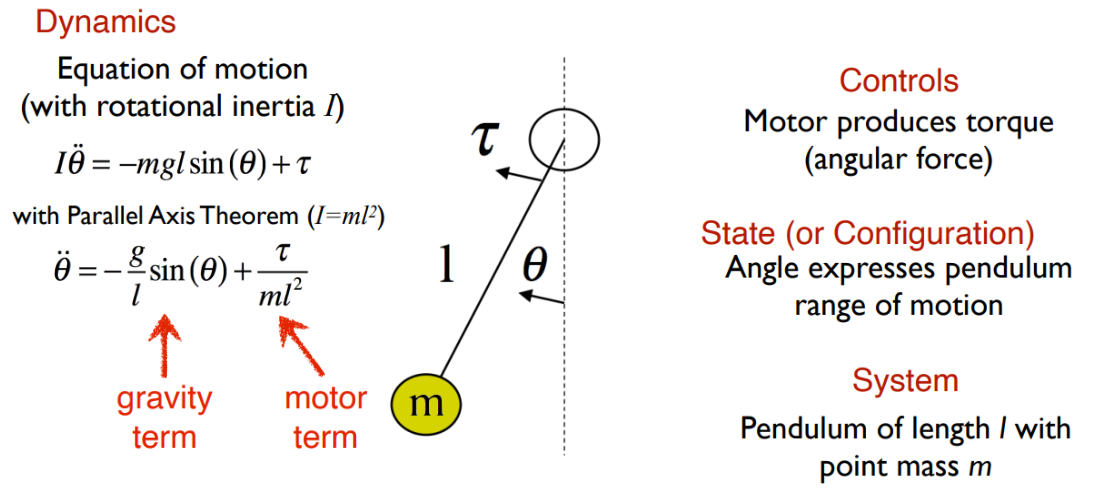
- where $\ddot{\theta} = \frac{d\dot{\theta}}{dt}$ as the rate of change of the velocity of the pendulum angle
- or $\ddot{\theta} = \frac{d\ddot{\theta}}{dt^2}$ as the rate of change of the rate of change of the pendulum angle
The equation of motion is derived from Lagrangian Dynamics for Pendulum. Lagrangian is kinetic energy minus potential energy $L = T-U$, and used to generate equation of motion as $\frac{d}{dt}\frac{\partial L}{\partial \dot{\theta}_i}-\frac{\partial L}{\partial \theta_i}=\tau_i$ where $\partial$ means partial derivative and $\frac{\partial L}{\partial \theta_i}$ is the rate of change of the Lagrangian with respect to only the $i^{th}$ DOF.
Now with the equation $\ddot{\theta}=-\frac{g}{l}sin(\theta)+\frac{\tau}{ml^2}$, the length and mass would stay constant, we need to think about how the angles evolve over time to calculate the motion. Then numerical integration kicks in.
Numerical Integration
What is numerical integration?
- Numerical Integration, namely numerical methods for ordinary differential equations, are methods used to find numerical approximations to the solutions of ordinary differential equations (ODEs).
Why do we care?
- The real world operates under Newtonian mechanics, use Newton’s equations of motion to model the change of a system over time, with numerical integration techniques and an initial position, we can approximate the system’s status at any specific time. We want to do it in simulation due to the high expense and low efficiency of experimenting on real robot in real world.
More into it ->
Euler Integration
Euler method is a first-order numerical procedure for solving ordinary differential equations (ODEs) with a given initial value.
- $y_{n+1}=y_n+hf(t_n, y_n)$ where h is the step size
How to estimate a future state $y(t_0+h)$?
- We use numerical integration over timestep duration,
next state-current state=integration over timestep - which is $y(t_0+h)-y(t_0)=\int_{t_0}^{t_0+h} f(t, y(t))dt$
Second-order state:
- Advance position using velocity: $y_{n+1} = y_n + \dot{y}_n\Delta_t$
- Advance velocity using acceleration: $\dot{y}_{n+1}= \dot{y}_n+ \ddot{y}_n\Delta_t$
However, Euler integration is not the best choice. The Euler method is a first-order method, which means that the local error (error per step) is proportional to the square of the step size, and the global error (error at a given time) is proportional to the step size.
Verlet Integration
Verlet Integration is a numerical method used to integrate Newton’s equations of motion.
- Initialize: $y_1 = y_0+h\dot{y}_0+h^2\frac{1}{2}a(y_0)$
- Advance position: $y_{n+1}\approx2y_n-y_{n-1}+a(y_n)\Delta t^2$
Velocity Verlet
A related, and more commonly used, algorithm is the velocity Verlet algorithm
- $y(t+\Delta t) = y(t)+\dot{y}(t)\Delta t + \frac{1}{2}a(t)\Delta t^2$
- $\dot{y}(t+\Delta t)=\dot{y}(t)+\frac{a(t)+a(t+\Delta t)}{2}\Delta t$
- Note that here we assume the acceleration $a(t+\Delta t)$ only depends on position $y(t+\Delta t)$
Runge-Kutta methods
Runge-Kutta methods are a family of implicit and explicit iterative methods, which include the Euler method (RK1), used in temporal discretization for the approximate solutions of simultaneous nonlinear equations.
- The most widely known member of the Runge–Kutta family is generally referred to as “RK4”, the “classic Runge–Kutta method” or simply as “the Runge–Kutta method”.
The “RK4” - Simpson’s Rule
The widely used version of fourth order Runge-kutta implements Simpson’s rule: $\int_a^bf(x)dx\approx\frac{b-a}{6}[f(a)+4f(\frac{a+b}{2})+f(b)]$
Express it as an integrator:
- Advance state: combination of integration trials at points with different tangents
- $y_{n+1}=y_n+\frac{1}{6}h(k_1+2k_2+2k_3+k_4)$
- Tangent at beginning of interval:
- $k_1 = f(t_n, y_n)$
- Tangent at trial midpoint $\frac{hk_1}{2}$:
- $k_2 = f(t_n+\frac{1}{2}h, y_n+ \frac{h}{2}k_1)$
- Tangent at trial midpoint $\frac{hk_2}{2}$:
- $k_3 = f(t_n+\frac{1}{2}h, y_n+ \frac{h}{2}k_2)$
- Tangent at trial end of interval:
- $k_4 = f(t_n+h, y_n+hk_3)$
- Advance time: $t_{n+1}=t_n+h$
This post is my notes from the class I am taking “ROB 511 Advanced Robot Operating System” offered by Prof. Chad Jenkins at University of Michigan.