Graph Search Algorithms in Path Planning
To build a robot that can go to a desired destination, we need to teach it how to plan the path. Path planning is about the best way to get from A to B. It allows robots to navigate the environments from previously constructed maps autonomously. A path planner finds a set of waypoints (or setpoints) for the robot to traverse and reach its goal location without collision, and there are many ways to do so.
We usually have a set of tools to respond accordingly to various situations. The common approaches we have:
- Bug algorithms: Bug[0-2], Tangent Bug
- Graph Search (fixed graph)
- Depth first search, Breadth first search, Dijkstra, A*, Greedy best-first search
- Sampling-based Search (build graph)
- Probabilistic Road Maps, Rapidly-exploring Random Trees
- Optimization (local search)
- Gradient descent, potential fields, Wavefront
In this post, we are going to explore the graph search methods.
Depth-first search (DFS)
Depth-first search is an algorithm for traversing or searching tree or graph data structures. The algorithm starts at the root node and explores as far as possible along each branch before backtracking.
DFS needs LIFO ordering, uses stack to keep exploring the latest added elements.
DFS is complete if the search tree is finite, meaning for a given finite search tree, DFS will come up with a solution if it exists. DFS is not optimal.
What does complete mean?
- If an algorithm is complete, it means that if at least one solution exists then the algorithm is guaranteed find a solution in a finite amount of time.
What does optimal mean?
- If no other search algorithm uses less time or space or expands fewer nodes, both with a guarantee of solution quality. The optimal search algorithm would be one that picks the correct node at each choice.
| Open Space | Has Obstacles |
|---|---|
 |
 |
| path length: 45.20 | path length: 150.20 |
| visited nodes: 453 | visited nodes: 1560 |
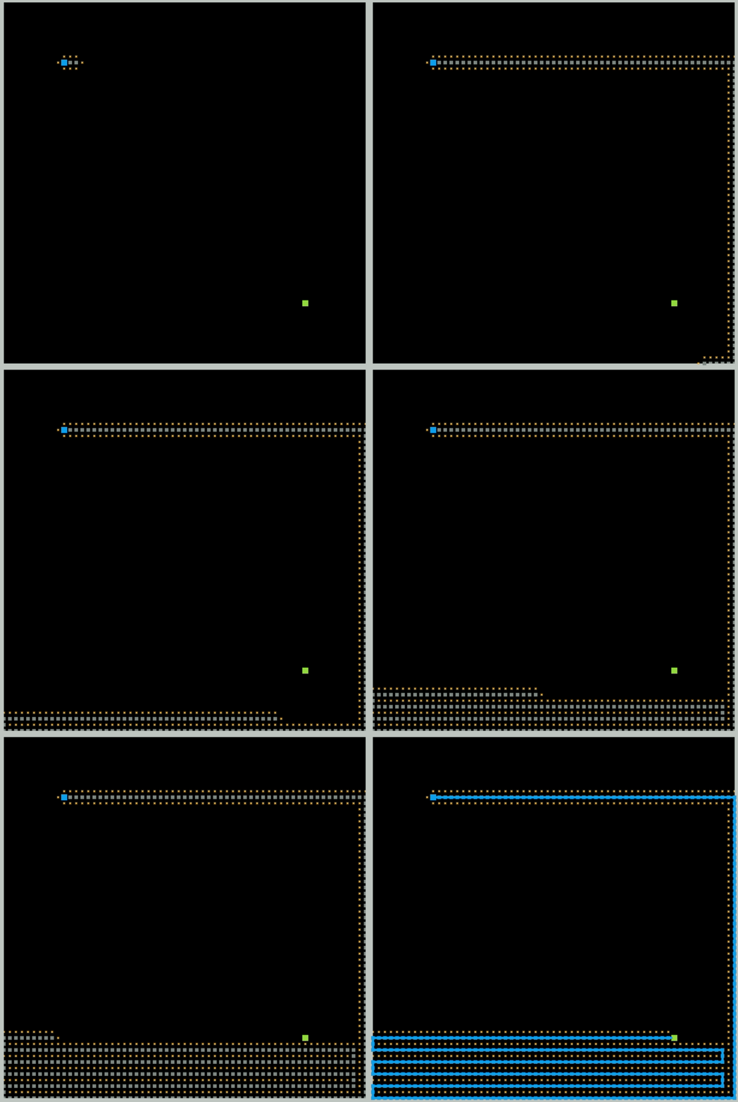
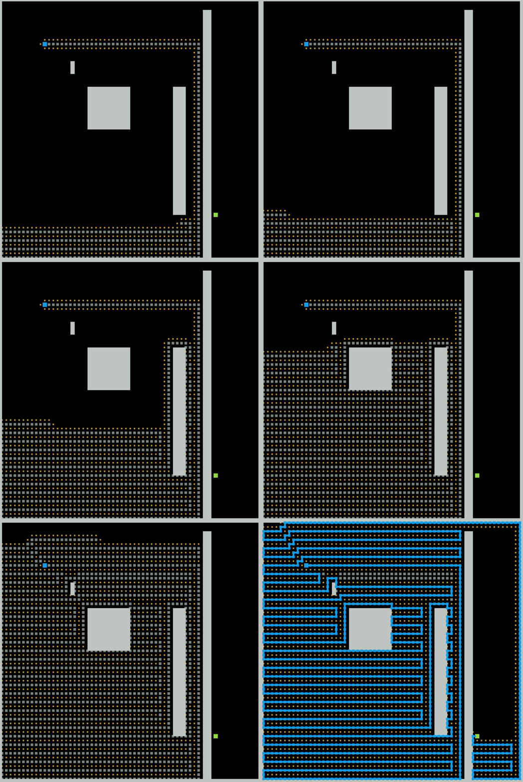
Based on my implementation, my DFS always goes right first, then clockwise when hitting a dead end. Since it is going without a clear direction, there is a lot of unnecessary exploration.
Breadth-first search (BFS)
Breadth-first search is an algorithm for searching a tree data structure for a node that satisfies a given property. It starts at the tree root and explores all nodes at the present depth prior to moving on to the nodes at the next depth level.
BFS needs FIFO ordering, uses queue to keep track of the child nodes that were encountered but not yet explored.
BFS is complete and optimal.
| Open Space | Has Obstacles |
|---|---|
 |
 |
| path length: 8.00 | path length: 9.80 |
| visited nodes: 3501 | visited nodes: 3235 |
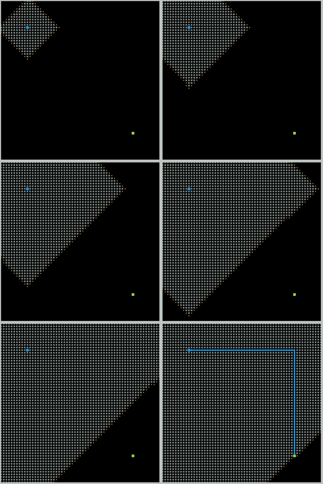
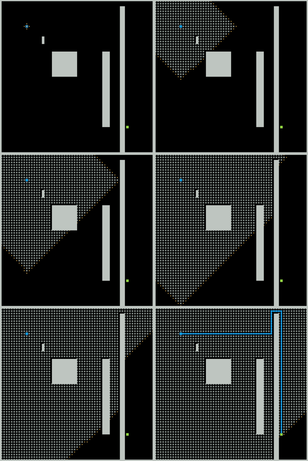
BFS also goes without a sense of where it should go, but it can always find the optimal path. Unlike DFS, the optimal solution is not guaranteed.
Greedy best-first search
Best-first search is a class of search algorithms, which explore a graph by expanding the most promising node chosen according to a specified rule. It is typically implemented using a priority queue.
Greedy best-first search is different with Best-first search. In the case of the greedy BFS algorithm:
- The evaluation function is $f(n)=h(n)$
- The Greedy Best-first Search algorithm first expands the node whose estimated distance to the goal is the smallest.
- Greedy BFS is neither complete nor optimal
| Open Space | Has Obstacles |
|---|---|
 |
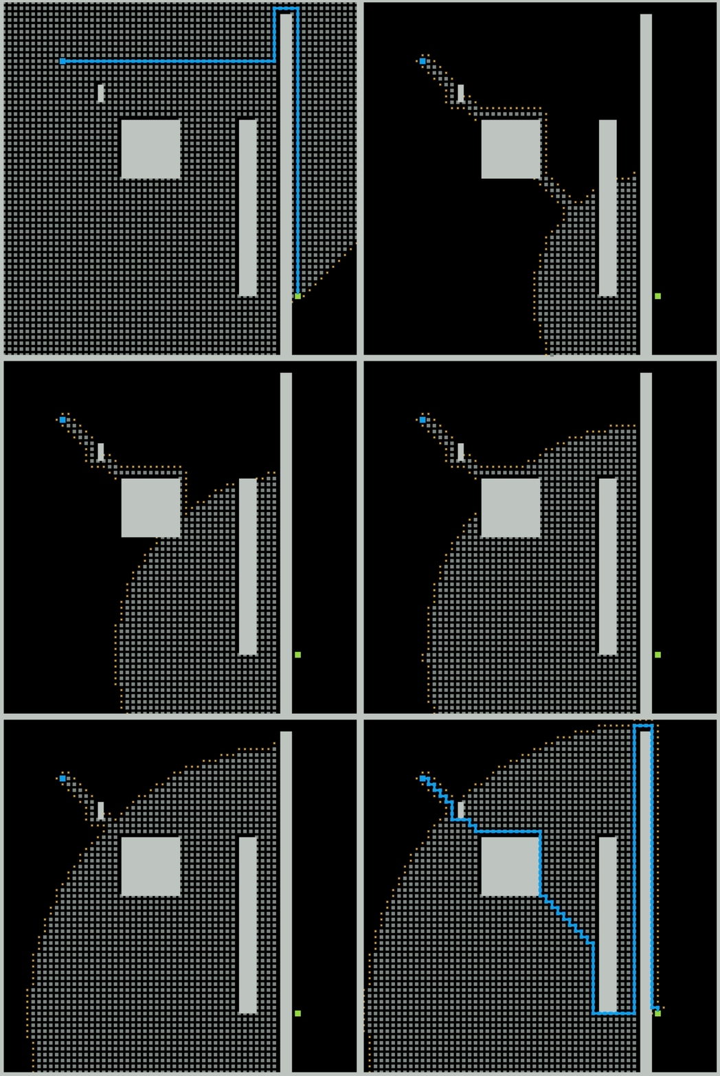 |
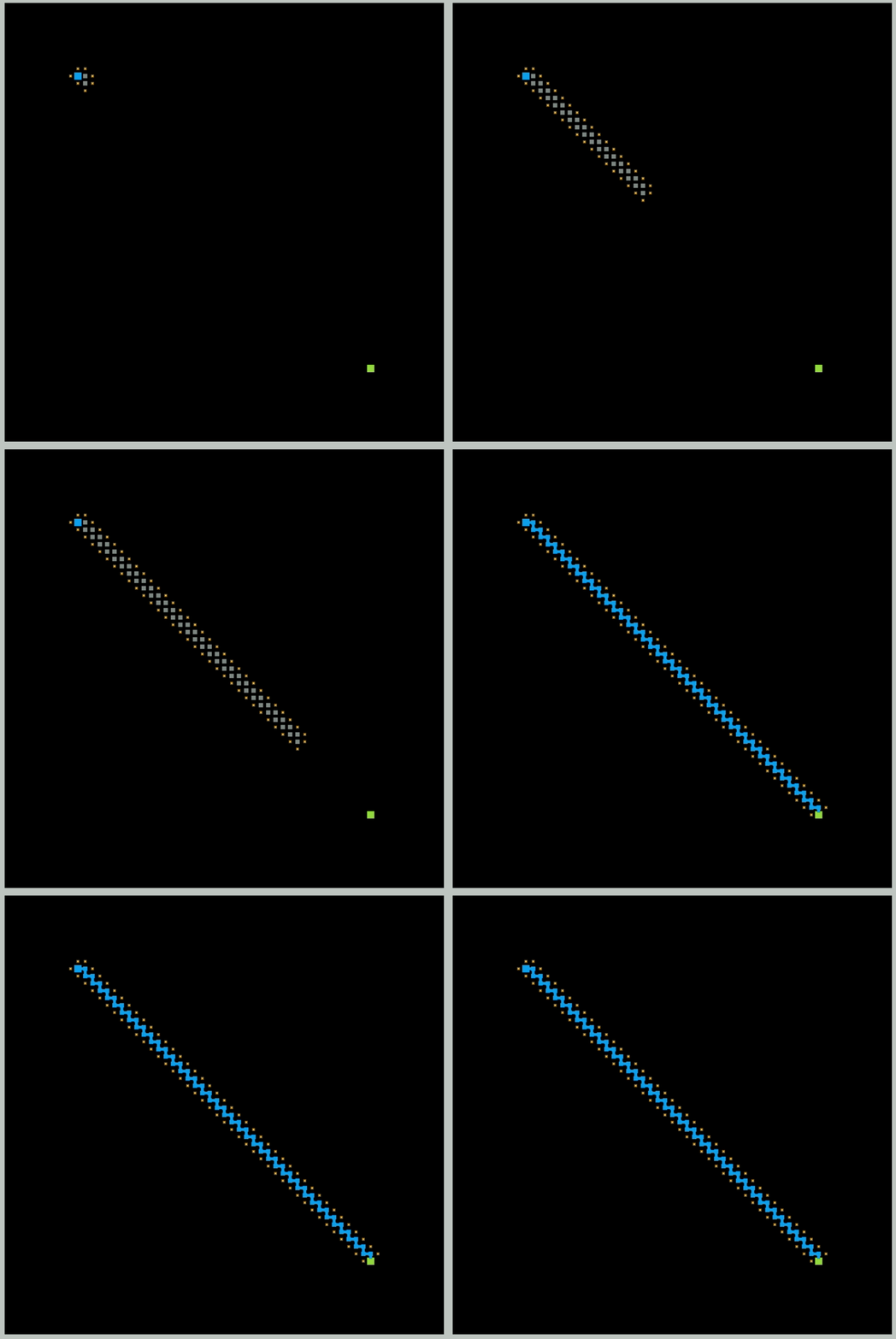
| path length: 8.00 | path length: 17.80 |
| visited nodes: 81 | visited nodes: 2074 |
As shown above, greedy best-first would perform very well when there are no obstacles, going directly to the goal is obviously the best way to navigate. However, when the map becomes complicated, it will pay the price for being “greedy.”
Best-first search and A* search are both informed search algorithm. A* is a kind of best-first search.
Depth-first search, Breadth-first search, and Dijkstra’s are all uninformed search algorithms. Uninformed search algorithms do not have additional information about state or search space other than how to traverse the tree, so it is also called blind search.
Dijkstra
Dijkstra’s Algorithm is used to find the shortest path from the source node to all other nodes in the graph. Starts by labeling all the distance to the source be infinity, then updated parent node and current cost for each node based on priority queue later, until no more update needed.
- Best explanation video
- The evaluation function is $f(n)=g(n)$
- g(n) is the cost of the path from the start node to n
| Open Space | Has Obstacles |
|---|---|
 |
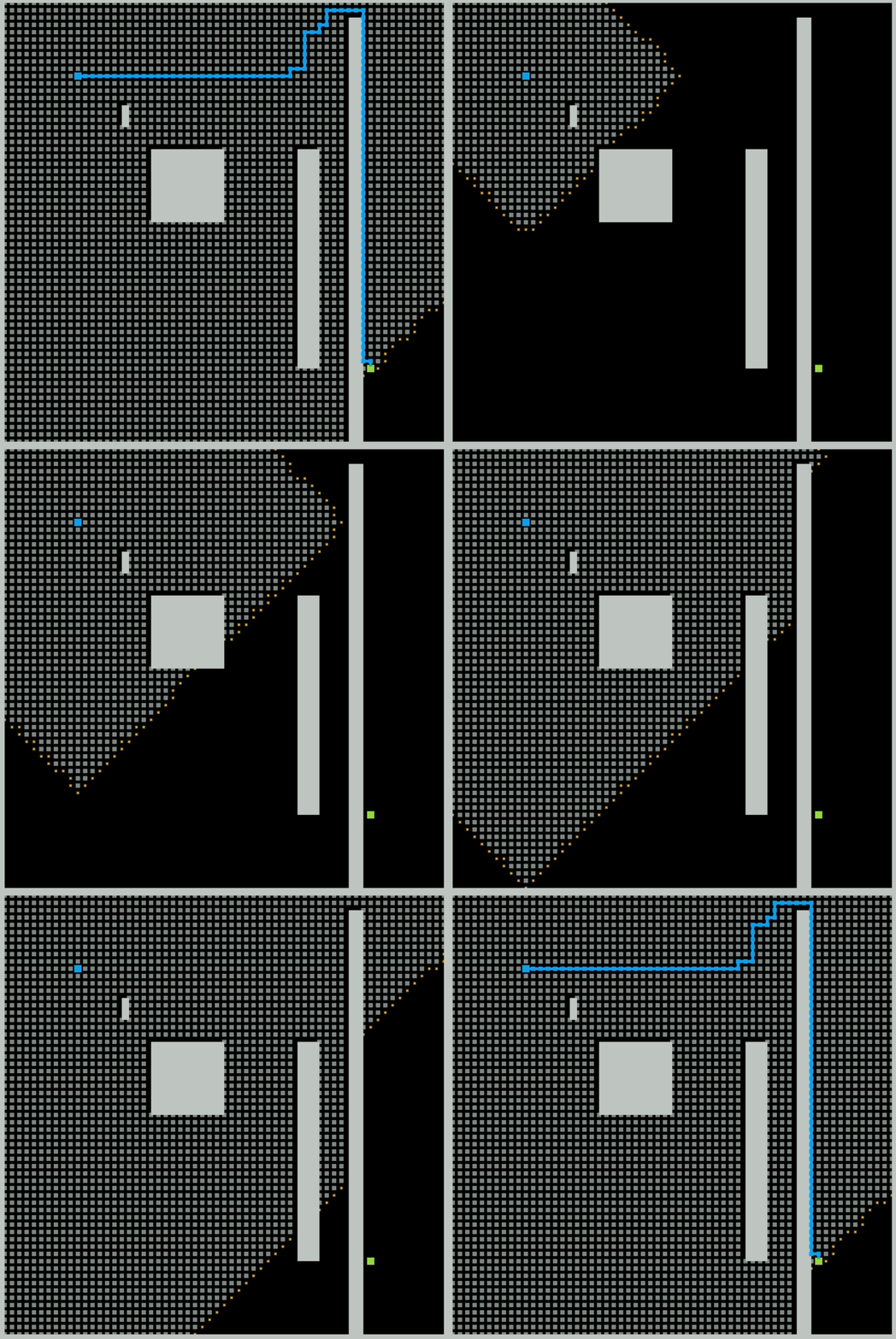 |
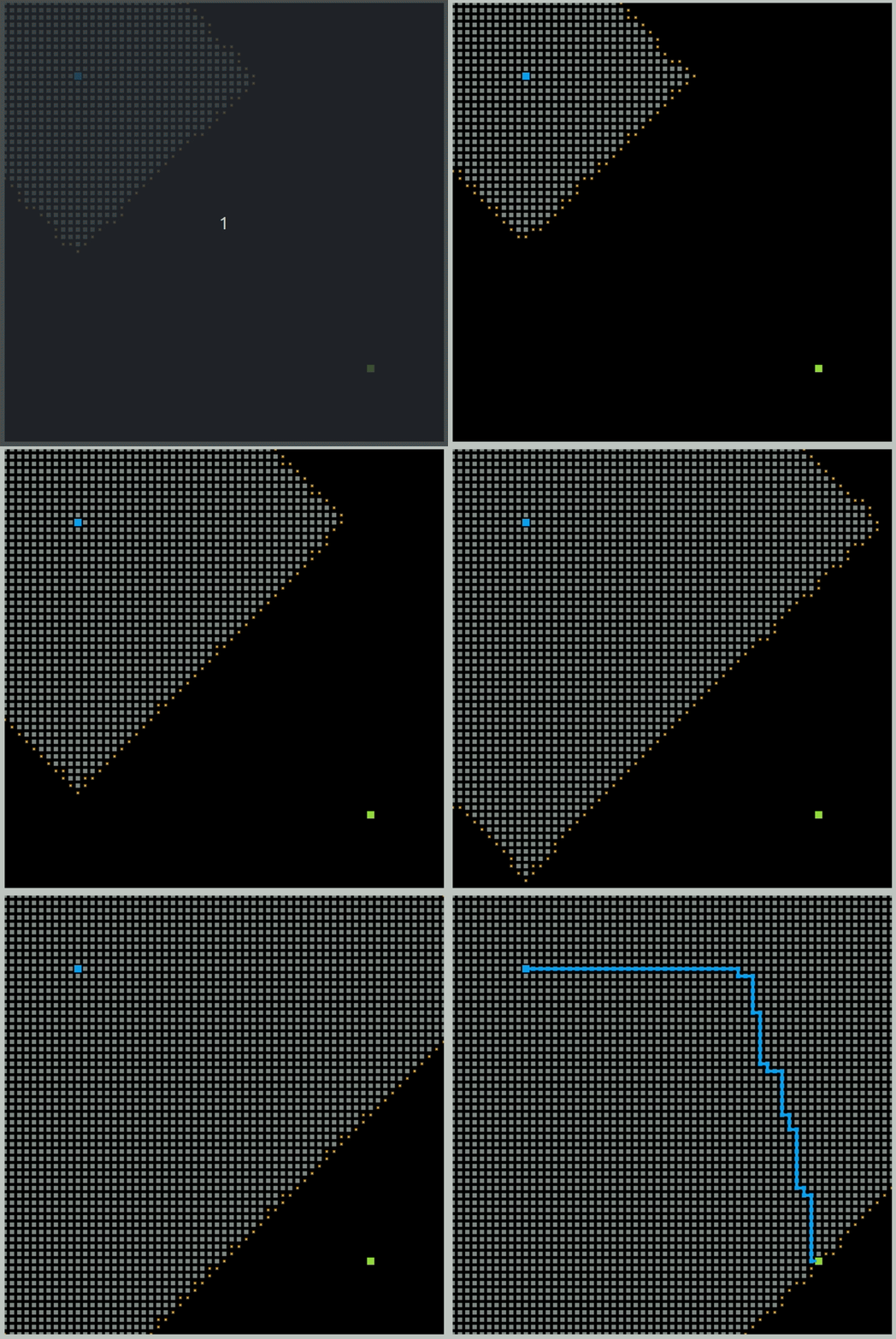
| path length: 8.00 | path length: 9.80 |
| visited nodes: 3495 | visited nodes: 3230 |
Dijkstra’s is based on a greedy approach, meaning we always choose local optimal solution at each step. The map above is a uniformly spaced, 4-connected grid map, meaning the cost to the adjacent node is always 1, such that the exploration process looks similar to a breadth-first search.
Dijkstra’s is good for finding shortest path from the source to all the others. But if we only want to find shortest path from one point to another, then Dijkstra’s might create unnecessary steps.
The famous A* algorithm is build upon this one. A* achieves better performance by using heuristics to guide its search. Compared to Dijkstra’s algorithm, the A* algorithm only finds the shortest path from a specified source to a specified goal, and not the shortest-path tree from a specified source to all possible goals. In pathfinding, we always choose A* over dijkstra.
A*
A* search algorithm infers the shortest path from a start to a goal location in an arbitrary 2D world with a known map (or collision geometry). A* requires an admissible heuristic, such as Euclidean distance or Manhattan distance, an educated guess of the cost to the goal.
- Best explanation video
- A* selects the path that minimizes $f(n)=g(n)+h(n)$ where
- n is the next node on the path
- g(n) is the cost of the path from the start node to n
- h(n) is a heuristic function that estimates the cost of the cheapest path from n to the goal.
- A* (which is a s best-first search) decays into Dijkstra’s algorithm when you use heuristic function h(v) = 0 for each v.
- A* is complete and optimal on graphs that are locally finite where the heuristics are admissible and monotonic.
- An algorithm is complete if it guarantees to return a correct answer for any arbitrary input (or, if no answer exists, it guarantees to return failure).
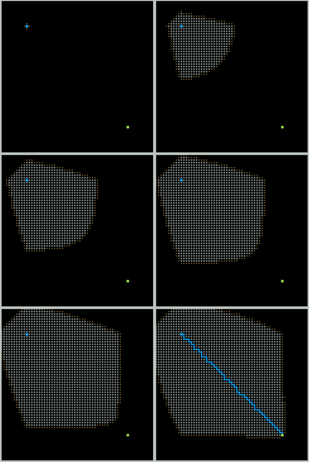
| Open Space | Has Obstacles |
|---|---|
 |
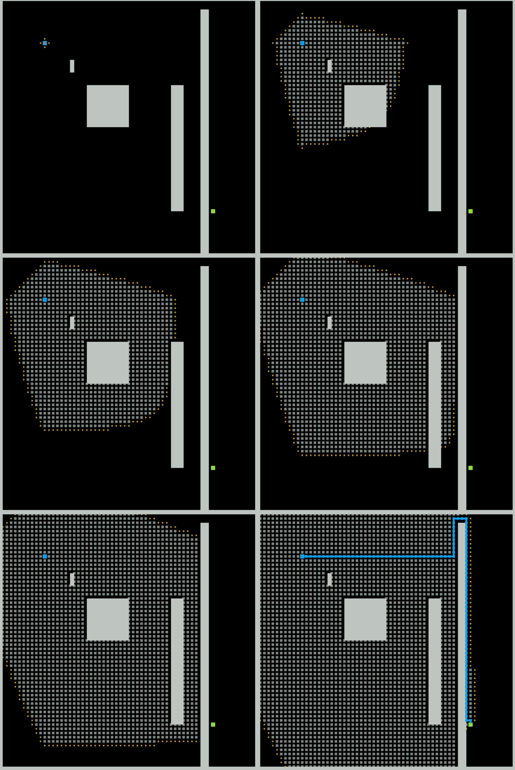 |
| path length: 8.00 | path length: 9.80 |
| visited nodes: 2242 | visited nodes: 2693 |
As shown above, the heuristic score guides the search process towards the goal for A* very well, the exploration is goal-oriented.
Conclusion
The gifs have shown that each algorithm has different characteristics, and there is no such algorithm that is all-purpose. Everyone has a situation where they are preferred.
A* can leverage both cost-to-come and cost-to-go, using heuristic value to guide the direction and use the g-value, namely cost-to-come, to correct the mistakes, unlike greedy best-first-search that doesn’t have past knowledge. However, the greedy best-first search is able to outperform all others when the space is relatively empty and there is no obstacle between the start and the goal.
DFS and BFS, as the uninformed algorithm, cannot compete with the informed algorithms in tests like path planning when the map is already constructed and relatively empty. However, BFS can always give the optimal solution even though it would spend a lot of time and memory searching. And DFS is more suitable when the goal is far from the source and when the map is more complicated, such as when solving a maze.
These gifs are generated from my coursework from the class I am taking “ROB 511 Advanced Robot Operating System” offered by Prof. Chad Jenkins at the University of Michigan. The interface credits to the course team.