PID Control

Motivation

The importance of control system is apparent. The control systems are everywhere in our life: when we want the air conditioner keeps the room temperature at 70F, when we want the fridge stays cool without freezing the veggies, and when we want the car to drive at a certain speed without stepping on the accelerator all the time, we have a control system there helping us.

A Cruise Control System consists of:

• Plant (car)
• Sensor (wheel speed sensor)
• Actuator (engine)
• Reference (drive at 35 mph)
• Disturbance (slope of road)
• Embedded processor (controller)

From robotics’ perspective, control is one of the most important aspects of robotics because it is the process by which a robot’s behavior is regulated and optimized. Control is essential in order to ensure that the robot can perform tasks accurately, efficiently, and safely.

In this post, we are going to discuss how to desgin a controller for a system.

Terminology

Specific controller design requirements:

• Stability: The controller and the plant should be (internally and BIBO) stable.
• Reference Tracking: System output tracks the desired reference command. In particular, the system output should follow reference commands with small overshoot and steady-state errors. In addition, the system should respond quickly, i.e. the rise and settling times should be small.
• Disturbance Rejection: The controller should be designed so that disturbances have a small effect on tracking.
• Actuator Effort: The input should remain within allowable levels.
• Noise Rejection: Since the controller relies on a measurement/sensor in most cases, it is required that any measurement inaccuracies have a small effect on tracking.
• Robustness to Model Uncertainty: The controller must be robust, i.e. insensitive, to model errors introduced by this simplified model.

What is ODE/Transfer Function?

• In control systems, transfer functions and ordinary differential equations (ODEs) are both used to model and analyze the behavior of a system.
• Transfer functions are commonly used to design controllers that can modify the system’s behavior in a desired way. It is obtained by applying a Laplace transform to the differential equations describing system dynamics, assuming zero initial conditions.

nth order nonlinear ODE:

\[y^{[n]} = f(y(t), \dot{y}(t), ..., y^{[n-1]}(t), u(t), \dot{u(t)}, ..., u^{[m]}(t))\]

nth order linear ODE:

\[a_ny^{[n]}(t)+a_{n-1}y^{[n-1]}(t)+...+a_1\dot{y}(t)+a_0y(t) = b_mu^{[m]}(t)+...+b_1\dot{u}(t)+b_0u(t)\]

Transfer function:

\[G(s) := \frac{b_ms^{m}+...+b_1s+b_0}{a_ns^n + a_{n-1}s^{n-1}+ ... + a_1s + a_0}\]

What is Initial Condition (IC)?
Initial condition refer to the value of the output and the (n-1) derivatives of the output at time t = 0. Zero initial conditions mean that the output and its (n-1) derivatives are 0 at t = 0. For example: $y(0)=0, \dot{y}=0, …, y^{[n-1]}(0)=0$.

Non-linear model is more accurate, linear model has properties (superposition, time-invariance) enable more direct theoretical analysis. When physical phenomena are modeled with non-linear equations, they are generally approximated by linear differential equations for an easier solution. Thus we use linearization to approximate non-linear ODE by linear ODE.

What is Linear Time-Invariant (LTI) System?

LTI system satisfies:

1. Superposition: scaling and additivity
   $u_1(t) \rightarrow y_1(t), \quad u_2(t) \rightarrow y_2(t)$
   $u_3(t) = a_1u_1 + a_2u_2 \rightarrow y_3 = a_1y_1 + a_2 y_2$

2. Time invariance
   $u(t) \rightarrow y(t), \quad u(t-c) \rightarrow y(t-c)$

What is system response?

In control systems, the system response refers to the output of a system as a function of time, given a specific input signal. The system response can be decomposed into two components: the free response and the forced response.

• Free response: input u(t) = 0 for all t >= 0
  • The free response can be thought of as the natural behavior of the system, in the absence of any external forcing.
• Force response: input u(t) != 0 for all t >= 0
  • The forced response is the component of the system response that is directly influenced by the input signal. It represents the effect of the input on the system’s output.

Transfer function $ G(s) := \frac{b_ms^{m}+…+b_1s+b_0}{a_ns^n + a_{n-1}s^{n-1}+ … + a_1s + a_0} $

• Pole/Root of G(s) is the solution of the characteristic equation: $a_np^n + a_{n-1}p^{n-1}+ … + a_1p + a_0 = 0$
• Zero of G(s) is the solution of: $b_mz^{m}+…+b_1z+b_0=0$
  • A zero in LHP: 1) Increase overshoot 2) Decrease rise time 3) No effect on settling time
  • A zero in RHP: 1) Cause undershoot 2) No effect on settling time
• DC gain or steady-state gain is $G(0)=\frac{b_0}{a_0}$

In control systems, it is often desirable to analyze the system response to various input signals. For example, if the input signal is a step function, the step response can be used to determine how the system behaves when it is suddenly subjected to a change in input. Alternatively, if the input signal is a sinusoidal function, the sinusoidal response can be used to determine the system’s frequency response, which is the system’s output as a function of input frequency.

First-order step response
A stable first-order system has step response that converges to the final value with neither overshoot nor oscillations.

Features:

1. Stable if root is in the LHP
2. No overshoot
3. Time constant: $\tau=\frac{1}{|{s_1}|}$
4. Settling time: $3\tau=\frac{3}{|s_1|}$
5. Final value: $\bar{y}=G(0)\bar{u}$, $\bar{u}$ is the input at equilibrium

Second-order step response
Consider the second-order system:
$\ddot{y}(t)+a_1\dot{y}(t)+a_0y(t)=b_0u(t), \quad y(0)=0, \dot{y}(0)=0, u(t)=1 $

The system is stable if and only if $a_1, a_0 > 0.$

For stable systems, $\ddot{y}(t)+2\zeta \omega_n \dot{y}(t)+\omega_n^2 y(t)=b_0u(t)$.

• $\omega_n$ is natural frequency (rad/sec)
• $\zeta$ is damping ratio (unitless).
  

Two poles are given by $s_{1,2}=-\zeta \omega_n \pm \omega_n \sqrt{\zeta^2-1}$, thus there are 3 cases depending on $\zeta^2-1$:

• Overdamped, $\zeta \geq 1$: roots are real and distinct
• Critically damped, $\zeta = 1$: roots are real and $s_{1,2}=-\zeta \omega_n$
  • Over/Critically damped solutions looks similar to the first-order response.
• Underdamped, $\zeta < 1$: roots are a complex conjugate pair. $s_{1,2}=-\zeta \omega_n \pm j\omega_n \sqrt{1-\zeta^2}$
  • Underdamped solution has overshoot and oscillations

Features:

• Final value: $\bar{y}=G(0)\bar{u}$
  • When u(t) = $\bar{u}$ and y(t) -> $\bar{y}$, all derivatives go to zero.
• Time constant: $\tau = \frac{1}{\zeta \omega_n}$
  • If the system is underdamped, calculate the zeta and omega, then calculate the time constant.
  • If the system is overdamped, we have to compute the poles and use the poles to calculate the time constant, like in a first-order system. And in this case, we should choose the root that is the smallest regarding the dominant pole approximation.
• 5% Settling Time: $T_s=\frac{3}{\zeta \omega_n}$
• Peak Overshoot: $M_p=e^{-\pi \frac{\zeta}{\sqrt{1-\zeta^2}}} \quad M_p=\frac{y(T_p)-\bar{y}}{\bar{y}}$
  • Mp a percentage, it is the peak-final value divided by the final value. So if the final value is 2, Mp is 0.35, then the peak is actually 2.7 because 2.7-2/2 = 0.35.
  • Only holds for second-order functions with no zeros.
• Rise Time: $T_r=\frac{\frac{\pi}{2}+sin^{-1}(\zeta)}{\omega_d}$
  • When there is overshoot, the time it takes to first reach the final value. If there is no overshoot, the rise time would be infinite.

Higher-order system
When analyze higher order system, we can use a method called Dominant Pole Approximation. It is a method for approximating a (more complicated) high order system with a (simpler) system of lower order if the location of the real part of some of the system poles are sufficiently close to the origin compared to the other poles.

• The approximation is accurate if the dominant pole(s) is significantly slower than the remaining poles. (Dominant pole time constant if 5x larger than other poles)

Stability

Internal Stability

• An LTI system is internally stable if the free response returns to zero for any initial condition. Note here that it doesn’t matter what the initial conditions are, if the system is stable, then it will converge to the final value.
• A linear system is internally stable if and only if all poles are in the LHP.

BIBO Stability

• An LTI system is bounded-input, bounded-output (BIBO) stable if the forced response output with zero ICs remains bounded for every bounded input.
• A minimal, linear system is BIBO stable if and only if all poles are in the LHP.

For minimal LTI systems, the two types of stability (internally and BIBO) are equivalent.

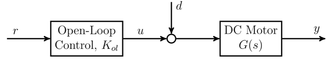
Open-loop Control

The difference between open-loop and closed-loop is that open-loop doesn’t have feedback.

Open-loop control can be effective if the plant is stable, the disturbances are small, and the model is accurate. If any of these conditions fail, then open-loop control will either fail to achieve stability (if the plant is unstable) or will not provide accurate tracking.

\[u(t)=K_{ol}r(t)\]

Closed-loop Control

The core of closed-loop controller is it acts based on error = desired - measured.

P Control

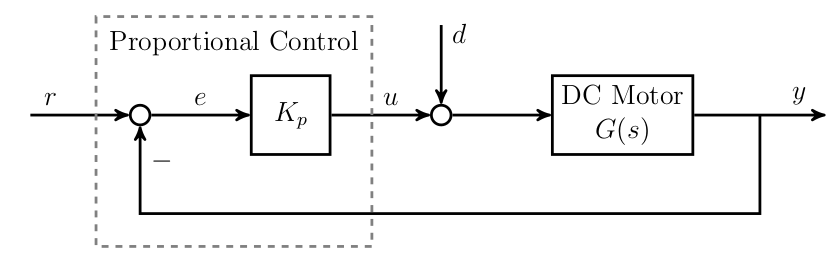
Proportional control sets input to be proportional to the error.

\[u(t)=K_pe(t)=K_p(r(t)-y(t))\]

• where u is input, e is error, r is reference, y is measured output, Kp is the gain to be selected.

If we substitude the equation above into a first-order system, we have:

\[\dot{y}(t)+(a_0+b_0K_p)y(t)=(b_0K_p)r(t)+b_0d(t)\]

• where d is disturbance
• Since the root is $s = -(a_0+b_0K_p)$, larger Kp yields faster response.
• However, even if y(t) is close to ybar, it can never reach reference due to the disturbance. Increase Kp could have better reference tracking and disturbance rejection, however, has a chance to exceed input limit and excite unmodeled dynamics.
• There will always be some error in steady-state when using only P control

PI Control

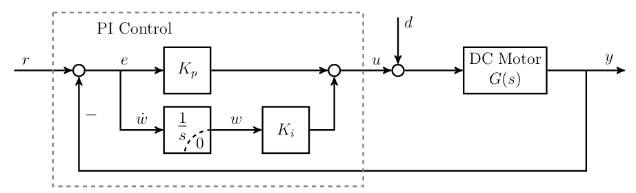
PI controller sets input to be proportional to 1) the error and 2) the integral of the error

1. The initial transient is dominated by the proportional term, while the steady state is dominated by the integral term.
2. Integral control will always achieve zero error in a steady state (assuming the system is stable and reaches a steady state).

\[u(t)=K_pe(t)+K_i \int_0^t e(\tau)d\tau\]

• P-Term: Reacts to present (current error) and dominates during the initial transient.
• I-Term: Reacts to past (integral of error) and dominates during steady-state.

PD Control

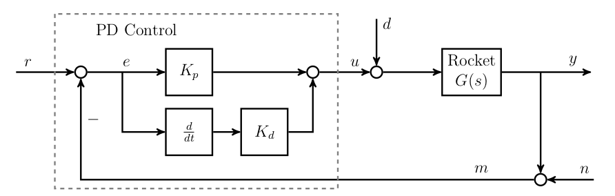
PD controller sets input to be proportional to 1) the error and 2) the derivative of the error

• Some plants cannot be stabilized by P or PI control which motivates the use of PD.
• A basic implementation of PD control will amplify noise. The common implementations use a “smoothed” derivative or direct measurement of the derivative of the output.

\[u(t)=K_pe(t)+K_d\dot{e}(t)\]

• P-Term: Reacts to present (current error)
• D-Term: Reacts to future (derivative of error) i.e. e could indicate the direction the error is headed. Has no effect on steady-state
  • If the derivative is positive, then we could expect the error would grow, if the derivative is negative, then the error would decrease.
  • When the plant is in a steady state, the error would be 0. Such that the D-term would only affect the transient.

Rate feedback implementation

$u(t)=K_p(r(t)-y(t))-K_d\dot{y}(t)$

This implementation doesn’t differentiate the reference, thus the rapid change in the reference command do not cause large control inputs. The term $-K_d\dot{y}(t)$ called rate feedback.

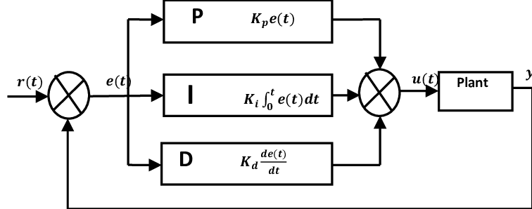
PID Control

PID Controller:

\[u(t)=K_pe(t)+K_i \int^t_0e(\tau)d\tau+K_d\dot{e}(t)\]

How to tune PID gains

1. Start all gains at zero : Ki = Kd = Kp = 0
2. Increase P gain Kp until system roughly meets desired state, overshooting and oscillation about the desired state can be expected
3. Increase damping gain Kd until the system is consistently stable. Damping stabilizes motion, but system will have steady state error
4. Increase integral gain Ki until the system consistently reaches desired
5. Refine gains as needed to improve performance
6. Test from different states

Miscellanea

• Servo is short for servomechanism, is an automatic device that uses error-sensing negative feedback to correct the action of a mechanism. Servos can be used to generate linear or circular motion, depending on their type.

---

Part of this post belongs to my notes from a class I have taken, “EECS 460: Control Systems Analysis and Design,” offered by Prof. Peter Seiler at the University of Michigan.