Forward Kinematics and Inverse Kinematics

Linear Algebra and Coordinate Frames (February 23, 2023)
Forward Kinematics (March 15, 2023)
Inverse Kinematics (April 2, 2023)

Linear Algebra and Coordinate Frames (February 23, 2023)

In Robotics, each part of the robot’s body might has its own coordinate system. Matrix transformations are used to transform coordinate systems between the bodies and joints. And here is where linear algebra kicks in.

Linear algebra, which deals with linear equations and linear mappings in the vector space, is used for modern presentations of geometry. It is essential for representing frames of reference, rotation, translation, and general 3D homogeneous transforms.

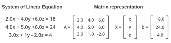
If #unknowns > #equations, it is an underdetermined system, usually with infinite solutions
If #unknowns < #equations, overdetermined system, usually with no solutions
If #unknowns = #equations, usually has a unique solution

2D Example

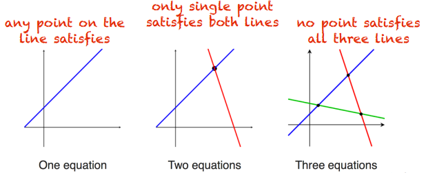
Coordinate spaces

How to represent coordinates spaces as systems of linear equations? - Vector

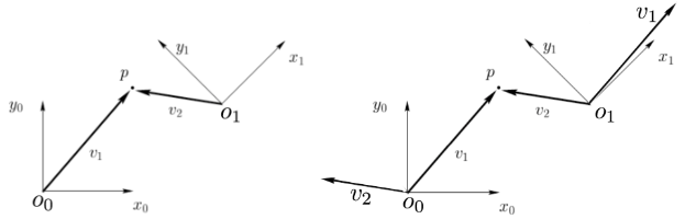
Two coordinate frames $o_0x_0y_0$ and $o_1x_1y_1$, and a point $p$ shown in the left image.
The location of point $p$ can be described with respect to either coordinate frame
- $p^0 = [5, 6]^T$ and $p^1 = [-2.8, 4.2]^T$
The vector $v_1$ is direction and magnitude from $o_0$ to $p$, and $v_2$ is from $o_1$ to $p$.
- $v_1^0 = [5,6]^T$ - vector 1 in frame 0
- $v_1^1 = [7.77,0.8]^T$ - vector 1 in frame 1

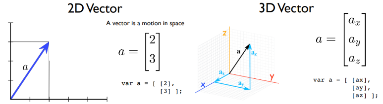
Vector operations

Addition and Subtraction

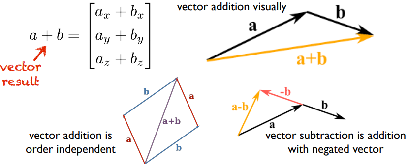
Magnitude and Unit Vector

The magnitude of a vector is the square root of the sum of squares of its components:
- $\left | a \right | = \sqrt{a_1^2+a_2^2+\cdots +a_n^2}$
A unit vector has a magnitude of one. Normalization scales a vector to unit length.
- $\hat{a}=\frac{a}{\left | a \right |}$

Dot Product

$a \cdot b= a_xb_x+a_yb_y+a_zb_z=\left | a \right |\left | b \right | \cos(\theta)$
- Dot product gives scalar result, it measures the similarity in direction of two vectors.
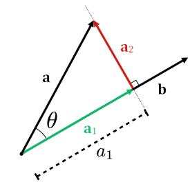
Dot products related to projections onto vectors. Scalar projection of one vector onto another:
- $a_1=\left | \mathrm{a} \right |\cos(\theta) = \mathrm{a} \cdot \frac{b}{\left | b \right |}= a \cdot \hat{b}$
Vector projection is $\mathrm{a}_1=a_1\hat{b}$
The difference is that $\mathrm{a}_1$ is a vector, and $a_1$ is a scalar. The scalar projection is using dot product, the vector projection is multiplied by a scalar.

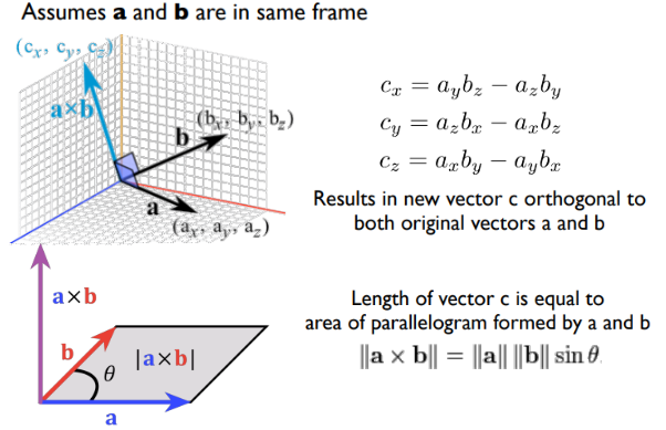
Given two vectors, how to compute a vector orthogonal to both? - Cross Product

Cross Product

Cross product denoted by $\times$, should not be confused with the dot product (projection product) which denoted by $\cdot$.

Given two linearly independent vectors $a$ and $b$, the cross product, $a \times b$ (read “a cross b”), is a vector that is perpendicular to both $a$ and $b$, and thus normal to the plane containing them.

Matrix operations

Matrix-vector multiplication

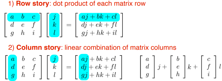
Matrix multiplication

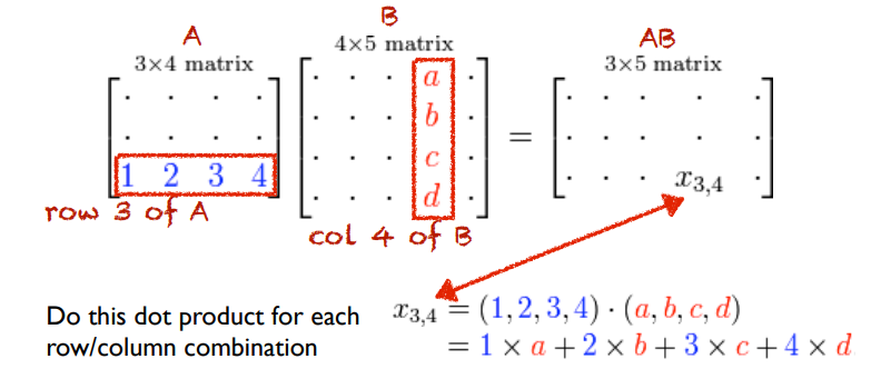
Notes:

Multiplying (MxK) matrix with a (KxN) matrix will produce an (MxN) matrix
Matrix multiplication is not commutative: AB != BA

Resource

Great tutorial series on Linear Algebra by 3blue1brown.

Forward Kinematics (March 15, 2023)

Robot Kinematics:

Goal: Given the structure of robot arm, we can compute
- Forward Kinematics: inferring the pose of the end-effector, given the state of each joint.
- Inverse Kinematics: inferring the joint states that are necessary to reach a desired end-effector pose.

Kinematic Foundations

Here is an example of an articulated robot. Articulated robot is a robot with rotary joints (e.g. a legged robot or an industrial robot). Articulated robots can range from simple two-jointed structures to systems with 10 or more interacting joints and materials.

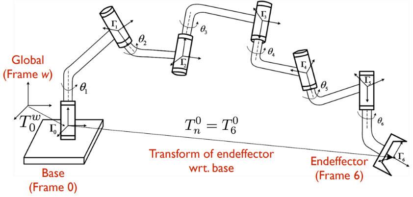
Forward kinematics is many-to-one mapping of robot configuration to reachable workspace end effector poses.

Workspace is a 3D space defined in the global frame.
Configuration $(q)$ is the state of all joints in the kinematics chain, $q = {q_1, \cdots, q_n}$
Joint $(q_i)$ relates the motion of one link (child link) with respect to another link (parent). Joint motion affects the child link and all of its descendants. In the image above, Link 1 $\Gamma_1$ is a child of joint 1 $\theta_1$, and Link 0 $\Gamma_0$ is the parent of joint 1.
- $q_i=\theta_i$ if it is a revolute joint
- $q_i = d_i$ if it is a prismatic joint
Kinematic chain connects N+1 links together by N joints, with a coordinate frame on each link.
Configuration space (C-space): the space of all possible configurations
DOF (Degree of freedom) of a robot is the dimension of the robot’s C-space, which is the minimum number of real numbers needed to represent the robot’s configuration. A rigid body in three-dimensional space has six degrees of freedom (DOFs).
- Position: motion along the x, y, z axis
- Orientation: rotation around x(roll), y(pitch), z(yaw).

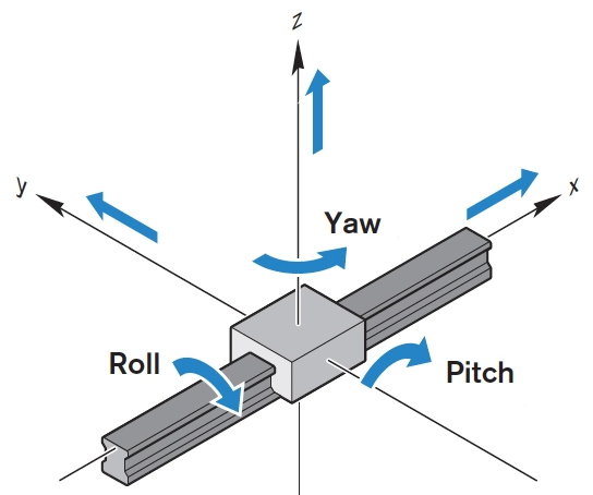
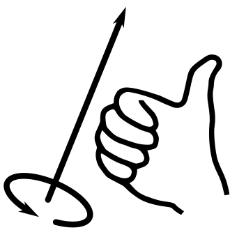
Right-hand rule

Coordinate conventions	A rotating body

Note that different application has different coordinate convention
To find the rotation direction, the right thumb pointing in the positive direction of the axis, and right fingers curled in the direction of rotation

The goal of forward kinematics is inferring the pose of the end effector given the state of each joint, thus we need to relate all the link’s own frame with each other, because every link considers itself to the center of the universe.

Then new questions arise, 1) how to represent the transforms? and 2) how to compute the transform to end effector?

First, we want to define the kinematics of a robot. Traditionally, we have Denavit-Hartenberg Convention. In recent years, we have URDF convention.

URDF stands for Unified Robot Description Format.
- URDF defined by its implementation in ROS (“Robot Operating System”), and ROS uses URDF to define the kinematics of an articulated structure. The structure is specified through XML. Kinematics represented as tree with links as nodes, joint transforms as edges.

Homogeneous transformation matrix

Homogeneous Coordinates

Homogeneous Coordinates are a system of coordinates used in projective geometry, just as Cartesian coordinates are used in Euclidean geometry.

Here is a great article of explanation and illustration.
- To make 2D homogeneous coordinates, we append an additional variable $w$ to the Cartesian coordinates $(X,Y)$, then we have $(x,y,w)$ in homogeneous coordinates. And reversely, the original $(X,Y)$ can be represented as $(\frac{x}{w}, \frac{y}{w})$. The value of $w$ would affect the size of the image.
  - Note here that the (x,y,w) is not a point in three dimensions like the Cartesian (x,y,z)
  - Motivation: In Euclidean space, two parallel lines will never intersect, but in projective space, two parallel lines can meet at the point of infinity. The third coordinate exists for one purpose only, and that is to add some points to the domain, namely, points at infinity. Sometimes, it is useful to think in terms of projective geometry.
    - For example, when we want to do translation and rotation at the same time. But translate operation is represented by matrix addition rather then multiplication, homogeneous coordinates will be helpful here.
- In 3D world, $w$ value works exactly the same as it does in 2D. A useful convention for 3D homogeneous coordinates is that we always set $w=1$ where the image doesn’t shrink or grow.
A Youtube video dives deeper into the topic.

2D space

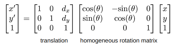
Composition of Rotation and Translation: by modifying both rotation matrix and translation vector into homogeneous coordinates, we are able to combine them into one single homogeneous transformation matrix, or a transformation matrix for short. Read from the right to left, we first do rotate and then translate.

Why not translate then rotate? Because $M = R\cdot T$ is different with $M = T\cdot R$.

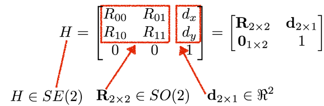
Special Euclidean group in two dimensions SE(2), where SO(2) means the group of rotations in two dimensions

Special Euclidean group, often denoted SE(n), whose elements are called rigid motions or Euclidean motions, that preserve the Euclidean distance between every pair of points. They comprise arbitrary combinations of translations and rotations, but not reflections.

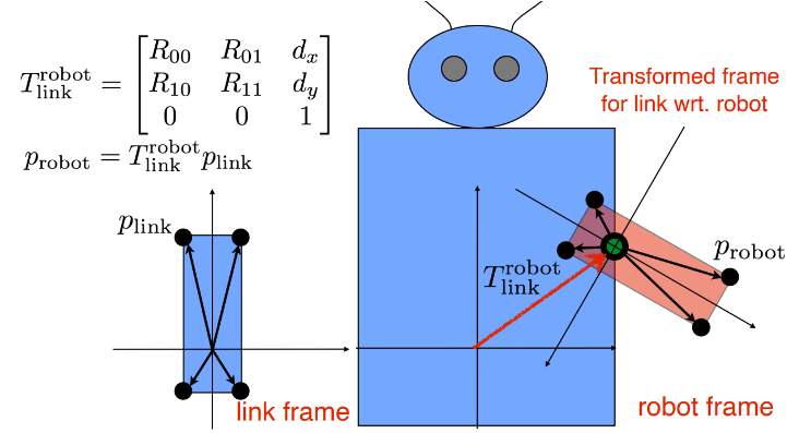
Example: Now we want to put an arm on the robot. By multiplying the transform matrix $T_{link}^{robot}$, we can find where the arm should at in the frame of the robot. If we analyze it step by step, firstly, rotate link frame by R, then translate link frame by d.

3D space

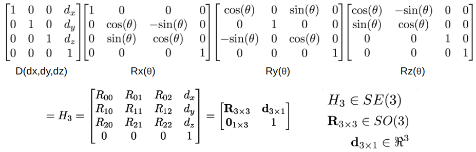
Here is the 3D homogeneous transform matrix. It consists of a translation matrix, and 3 rotation matrices relate to rotate along x,y,z axis. If you are familiar with pinhole camera model, this is the extrinsic matrix to map points from the world frame to the camera frame.

Axis-Angle Rotation and Quaternions

In the transformation matrix above, we use Euler Angles to express the rotation around x(roll), y(pitch), z(yaw).

However, it is problematic when rotate about each axis in order $R = R_x(\theta_x)R_y(\theta_y)R_z(\theta_z)$. Something called Gimbal lock would occur when 2 axes are rotated into alignment. It will reduce 3 DOFs to 2 based on the axis order.

Alternatives to present rotations:

Axis-angle representation which only valid in 3D space. It parameterizes a rotation in a three-dimensional Euclidean space by two quantities: a unit vector $e$ indicating the direction of an axis of rotation, and an angle $\theta$ describing the magnitude of the rotation about the axis.
- Example: (axis, angle) = ($[0, 0, 1]^T, \frac{\pi}{2}$), rotate along z-axis by 90 degrees
Quaternion, which is useful for describing orientation and computing rotations in 3D world for robotics.
- It is just a different way to describe the orientation of a body, not meant to be read directly, namely not as intuitive as the Euler angle. Quaternions are more numerically robust, so if we have access to it, we should choose it over Euler angles.
- ROS’s tf library has function from tf.transformations import quaternion_from_euler which can help us to do the conversion conveniently.

Quaternion conversion

Calculate quaternion from axis-angle representation:
- Concept

import math

def quaternion_from_axis_angle(axis, angle):
	"""
	Convert axis angle representation to quaternion representation

	Return [x, y, z, w] where w is the real number
	"""
	q = [0]*4
	q[0] = axis[0]*math.sin(angle/2)
	q[1] = axis[1]*math.sin(angle/2)
	q[2] = axis[2]*math.sin(angle/2)
	q[3] = math.cos(angle/2)

	return q

# Test:
axis = [0, 0, 1]
angle = math.pi/2
print(quaternion_from_axis_angle(axis, angle))

Now we have answered the question 1) how to represent the transforms?

The answer is by using transformation matrix.
The next question is how to compose these matrices hierarchically to compute transform wrt. world?

Matrix stack for FK computation

We need to transform along kinematic chain bringing descendants along, such that we can find where the end effector at in the world frame. The hierarchy is given by the URDF file.

Goal: compute transform of frame at each kinematic node into the world frame.
Approach: Compose transforms along kinematic tree using a stack data structure
- top of the stack is transform for current node
Code: Recursively alternate between link and joint to update transform at top of stack
- start with base link and global transform
- for each link, recurse over all children
- for each joint, compose rotational and translational effects and push it into the stack

Inverse Kinematics (April 2, 2023)

There are many ways to solve inverse kinematics, and can be categorized into two types:

Closed form (analytical) solution: a sequence or set of equations that can be solved for the desired joint angles, solves the whole system at once
- Speed: solution often computed in constant time
- Predictability: solution is selected in a consistent manner
Iterative (numerical) solution: Solved by optimization, minimize error of endeffector to desired pose
- Often in some form of Gradient Descent (a la Jacobian Transpose)
- Generality: same solver can be used for many different robots

Analytical solution

Using analytical method, each joint angle is calculated from the pose of the end-effector based on a mathematical formula. By defining the joint parameters and end-effector poses symbolically, IK can find all possible solutions of the joint angles in an analytic form as a function of the lengths of the linkages, its starting posture, and the rotation constraints.

There is no general analytical inverse kinematics solution.

All analytical inverse kinematics solutions are specific to a robot or class of robots, based on geometric intuition about the robot

Numerical solution

Using numerical solution, each joint angle is calculated iteratively using algorithms for optimization, such as gradient-based methods.

What is Jacobian?

Jacobian matrix is a matrix of partial derivatives.

The term “Jacobian” often represents both the jacobian matrix and determinants, which is defined for the finite number of function with the same number of variables. Here, each row consists of the first partial derivative of the same function, with respect to the variables. The jacobian matrix can be of any form. It may be a square matrix (number of rows and columns are equal) or the rectangular matrix(the number of rows and columns are not equal).

Jacobian Transpose

To have iterative solution, our goal is to move the endeffector to minimize error, where error means the difference between the goal state and current state.

We know that when we are at x = 0m and we want to get to x = 2m, we need to move in x-direction with certain velocity to minimize the error. Now the questions is, how are linear and angular velocity related? Since the way to move the end effector in x-direction is by rotating the angle (if using revolute joint).

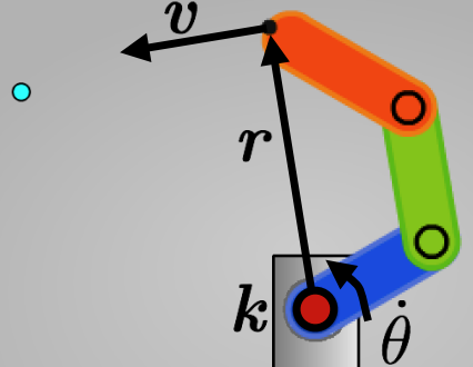
\[\omega = \dot{\theta}k \quad v = \omega \times r \quad v = \dot{\theta}k \times r\]

$\omega$: angular velocity of points in the frame wrt. axis k
$\dot{\theta}$: rotation speed of frame
$k$: joint rotation axis, could be [0, 0, 1] if the vector represents [x, y, z]
$v$: endeffector linear velocity
$r$: vector from joint origin to endeffector

We related the linear velocity and the angular velocity, however, what we want to know is how much change in the angle we need, now the LHS is the variable we know. To obtain joint angular velocity from endeffector linear velocity, we introduce Jacobian Transpose here.

\[\Delta \theta = (k \times r)^T \Delta x\]

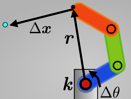
$(k\times r)$: Jacobian for joint i
$\Delta \theta $: Angular displacement for joint i
$\Delta x $: desired endeffector displacement

Such that to calculate the inverse kinematics, for each joint on the chain from the base link to the end effector, we firstly 1) Compute the Jacobian, then 2) Update joint angles using Jacobian transpose, finally 3) repeat the process until error minimized.

To minimize the error, we are going to use a method called Gradient descent.

Gradient descent

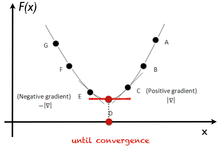
Gradient descent is a first-order iterative optimization algorithm for finding a local minimum of a differentiable function.

\[x_{i+1} = x_i - \gamma_i \triangledown F(x_i)\]

$\gamma_i $ is learning rate, it is the step size of each step
$\triangledown F(x_i)$ is the derivate of F(x) which is the slope of current position

Now our question becomes: What is the derivative of robot configuration? - Geometric Jacobian

Geometric Jacobian

Geometric Jacobian of the end effector is a 6-by-n matrix, where n is the number of degrees of freedom of the robot. The Jacobian maps the joint-space velocity to the end-effector velocity, relative to the base coordinate frame. The end-effector velocity equals:

\[V_{EE} = \begin{bmatrix} v_x\\ v_y\\ v_z\\ \omega_x\\ \omega_y\\ \omega_z \end{bmatrix} = J\dot{q} = J \begin{bmatrix} \dot{q_1} \\ \vdots\\ \dot{q_n} \end{bmatrix}\]

where $\omega$ is the angular velocity, $v$ is the linear velocity, and $\dot{q}$ is the vector of joint-space angle velocity.

$J$ consists of two 3-by-n matrices $J = \begin{bmatrix}J_v\J_w\end{bmatrix}$ as shown above. To calculate $J$ for each joint i, we have equations:

\[J_{vi} = (\{k_i\}^w - \{o_i\}^w) \times (\{p_{tool}\}^w - \{o_i\}^w)\] \[J_{\omega i} = \{k_i\}^w - \{o_i\}^w\]

Endeffector: ${p_{tool}}^w = T^w_n{p_{tool}}^n$ = the position of the end effector in world frame
Joint-axis endpoint: ${k_i}^w = T^w_i{k_i}^i$ = a point one unit along the joint axis from its origin, expressed in the world frame.
Joint origin: ${o_i}^w = T^w_i{o_i}^i$ = the origin of the joint in world frame
All the above variables are in world frame, T is the transformation matrix.

Error Minimization by Gradient Descent using Jacobian Transpose

We first calculate the error:

\[\Delta x_n = x_d - x_n\]

Then compute the step direction:

\[\Delta q = J(q)^T \Delta x\]

Finally perform the step direction:

\[q_{n+1} = q_n + \gamma \Delta q_n\]

Jacobian Pseudoinverse

What is Pseudoinverse? - answer

For a matrix A with dimensions N x M with full rank
- Left pseudoinverse for full column rank, meaning $N \geq M$, “tall” or square
  - $A^{-1}_{left} = (A^TA)^{-1}A^T$
- Right pseudoinverse for full row rank, meaning $N \leq M$, “wide” or square
  - $A^{-1}_{right} = A^T(AA^T)^{-1}$

function matrix_pseudoinverse(m) {
    // returns pseudoinverse of matrix m
    var row = m.length;
    var col = m[0].length;
    var m_trans = matrix_transpose(m);

    if (row >= col) {
        return matrix_multiply(numeric.inv(matrix_multiply(m_trans, m)), m_trans);
    } else {
        return matrix_multiply(m_trans, numeric.inv(matrix_multiply(m, m_trans)));
    }
}

Error Minimization by Jacobian Pseudoinverse